
shows the starting point (upside down) for a block of tau values in region F.
The image
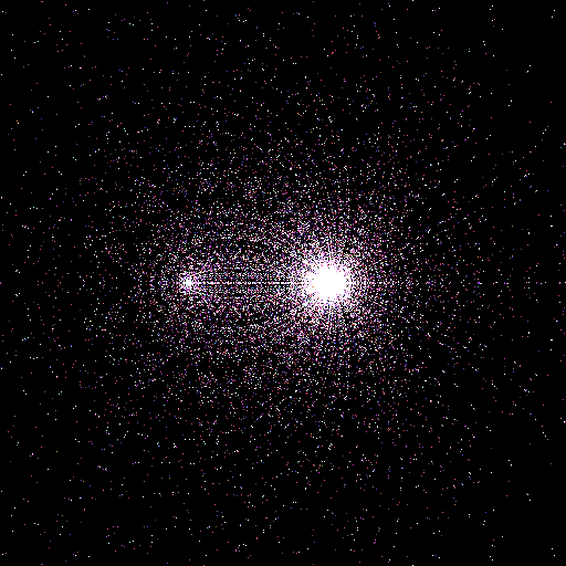
shows where those points end up after passing thru the function j(tau).
The range of values in this plot are:
The purpose of the "big float" project is to be able to compute the
number of points on an arbitrary elliptic curve over any basis (but
base 2 is the initial target) using complex numbers. This comes
from
all elliptic curves being defineable on Reimann surfaces which can
be
mapped to the complex plain.
I'll probably get burned out making it work, if anyone wants to
make it efficient I won't stop you :-)
The file bigfloat.h
contains the header info and creates the storage
data sizes. The fundamental
data type is FLOAT and COMPLEX is built
from it.
The file bigfloat.c contains the floating point basics, add, multiply and divide.
The file bigfunc.c
contains routines for computing high level functions. One routine computes
PI, another ln(2), x^m and one routine computes bessel functions J(n,x) and I(n,x)
for use as coefficients of exp and cosine functions. But they work for any input.
Also computes Chebyshev polynomials using MULTIPOLY described below.
The file
bigcomplex.c
contains the complex portion of the basics including add,
multiply
and divide. There is also cmplx_intpwr()
which takes a complex number to an arbitrary integer power. This
is the beauty of brute force (See Solinas, equation 24 in "Improved
Algorithms for Arithmetic on Anomalous Binary Cruves").
The exp_cmplx() function is busted, I'm still working on that.
The file
bigio.c
contains a routine to convert ascii to FLOAT.
Numbers
are input "backwards" because the exponent is more important than the
mantissa for back of the envelope calculations. The format is
E[s]xxxxxxxxx\t[s]xxxx-----.xxxxxx-------
The E (or e) is manditory, the sign [s] is optional, can be +, - or
not there, 0 to 9 digits for an exponent (no bug checking on that tho!)
\t is blank or tab (manditory or it does return an error)
another optional sign for the mantissa followed by any number
of digits, a decimal point and any more number of digits.
I just skip anything outside '0' - '9', no errors report for
garbage.
I can promise that this code has bugs! I will not complain about
help finding them. Thanks!
The file
multi_float.c
contains routines to deal with both power series and polynomial series.
These are subtly different, a power series only keeps low level terms
and drops off high order terms, a polynomial series keeps all terms.
The former is used to find coefficients of j(tau), the latter to compute
coefficients of Chebyshev polynomials.
The file
multi_mem.c
contains memory management routines for the power series and polynomials.
This is a home grown effort to get past bugs I had with Linux when trying
to glom up huge amounts of ram. Now I just allocate 40 to 100 Megabytes
and parse it out myself.
The file
multipoly.h
contains structures and macros used by the memory manager. This isn't so
easy to debug, but ddd can deal with it if I'm careful.
The file
joftau.c
puts it all together and computes the coefficients of j(tau), the
quintisential elliptic modular function.
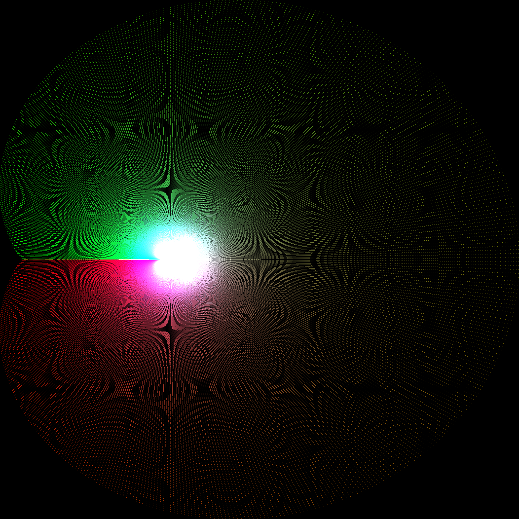
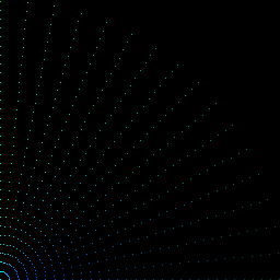
The following plots show various values of tau, taken from the region
F as defined by J. Silverman in "Advanced Topics in the Arithmetic of
Elliptic Curves". There are two groups of 2 plots. Each group contains
an "initial" shot of selected points in the complex plain, the initial
tau. The second picture of the group shows where those points map to
on the complex plain after passing thru the function j(tau).
The function j(tau) = 1/q + 744 + sum{ c_n * q^n } and q = exp(2*PI*i*tau)
The region F is between -1/2 and +1/2 on the real axis and all
imaginary values outside the unit circle. The colors follow from - real
as dark red and flow to + real as dark green, each fading into the other
smoothly. An index goes across the unit circle for each point for the
horizontal plot. The color blue goes from maximum intensity at the
unit circle to minimum intesity at the maximum. For group 1, the
maximum imaginary value is 1 + 2/pi. For group 2, the maximum imaginary
value is 1 + 1/2pi.
The image
shows the starting point (upside down) for a block of tau values in region F.
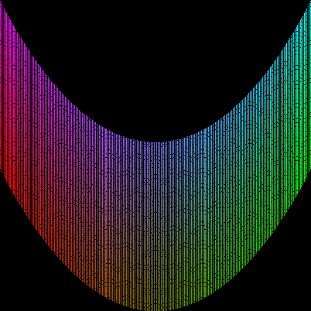
The image
shows where those points end up after passing thru the function j(tau).
The range of values in this plot are:
xfmin is
E+000000008 -0.73622231322385085926634970946152571381859403857472743143269675499885980035224940
yfmin is
E+000000008 -1.26238094472149050931740587985973402816596942673720194472356703552129312750445382
xfmax is
E+000000008 +1.49827197538546788420887407859444075028691369845306205654895456993792376732349189
yfmax is
E+000000008 +1.26238094472149050931740587985973402816596942673720194472356703552129312750390111
Here is the starting point
 (upside down).
Here is the resulting map
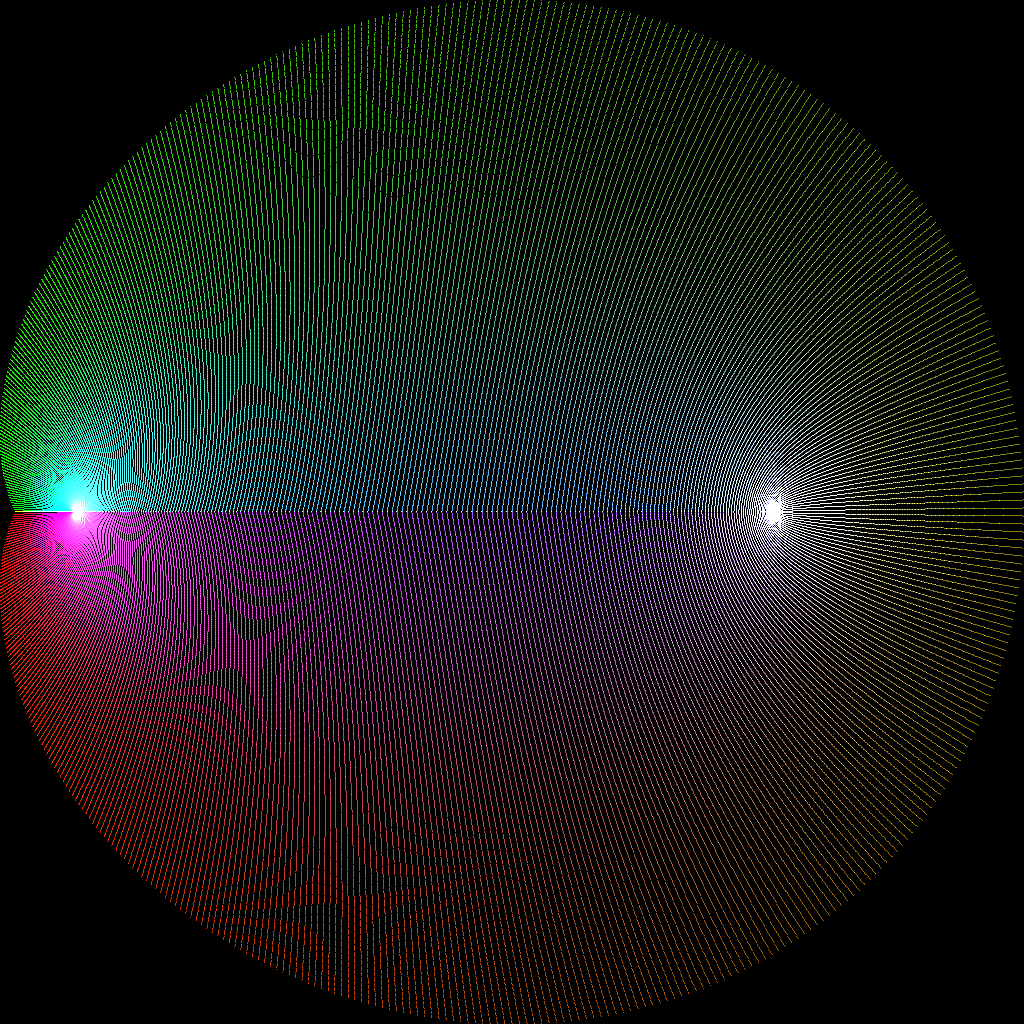
the range on this plot is
xfmin is
E+000000002 -1.83622468938171816894194073740056064470224111076645670806815000210227948943928982
yfmin is
E+000000003 -1.06599416826236086244051990169315766142354777038367386253689824467849631065120382
xfmax is
E+000000004 +0.23427318255569180380242306242150096690392370610061283770750494821952516636355670
yfmax is
E+000000003 +1.06599416826236086244051990169315766142354777038367386253689824467849631065009839
By following the colors from the start plot to end plot you can see how
j(tau) operates on tau in F. By going from group 1 to group 2, you can
"zoom in" on the functions. It is easy to see that for tau = i, you
get the point exp(2pi) + 744 and for tau = +/- 1/2 + iAcos(Pi/3) you get
0,0. To me it looks pretty cool.
Here are 2 plots from the many I have of the Weierstrass "rho" function.
This function takes 2 complex inputs called z and tau. Tau is the
same as above, z is an arbitrary point in the complex plane.
I take tau as a 64 by 64 bit grid in range unit circle to 10.0,
and use red to mark the real axis and green to mark the imaginary
axis as seen here.
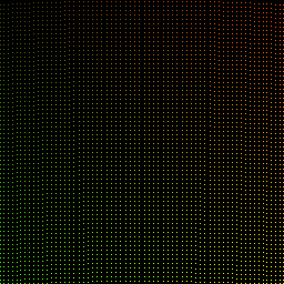
I use blue to mark off z radii in 32 steps and each angle (marked
in increasing green) is used to create a separate plot. The z source
is here:
z angles of PI/2 (pure imaginary)
 and 3*PI/32 for plots of rho are shown here.
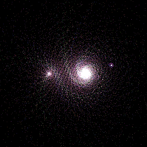
The pictures are centered on (0, 0) and have width 1.0
You can see a zoom sequence from width 100x100 down to about 1e-13 x 1e-13 here. It's about 850k of plots so it takes a while.
Here is another view of the same thing but the z plot looks like this
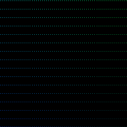
The following sequence is a view going thru several slices of constant real z. Tau is colored as above (bright green near unit circle and fading as imaginary increases, bright red for real tau = 1/2). You can see how tau figures into rho. Blue is bright where imaginary z is small, and fades as z gets larger. The range on this is 0..1 for both real and imaginary values of both tau and z. Check out this slice sequence.
For more information, send e-mail to Dr. mike.